


Treatment of Poultry Litter by Windrowing: Evaluation on Commercial Farms
Corina Bernigaud and Juan Martín Gange, from INTA (National Institute of Agricultural Technology) Experimental Station, Concepción del Uruguay, Argentina, discuss poultry litter management techniques. The aim of the two experiments discussed was to analyse the technique of windrowing poultry litter during clean down of commercial broiler houses under farm conditions. 27 September 2016
 14 minute read
 By:
By: 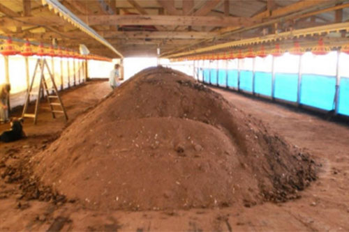
Temperature, windrow height and bacterial load (enterobacteria and sulphite-reducing anaerobes) were examined in these two experiments. The farmer's usual technique of windrowing the litter for 7 days, without turning or adding water, was used during the study.
Moisture, pH, Electrical Conductivity (EC), Total Carbon (C), Total Nitrogen (TN) and Total Phosphorus (TP) were also measured. The first, pooled samples from the whole pile were taken as the windrow was formed, and the last samples were taken at the end of the 7-day windrow period from the locations of the 12 temperature sensors. TN and TP samples were only taken from some of the locations at the beginning and end of the process.
Farm 1: details
The same litter was used for two flocks on this farm in the Department of Uruguay in Entre Rios; the first for 46 days and the second for 42 days. Trial duration was seven days.
100 m x 10 m house, orientated east-west, bedding of Eucalyptus shavings, automatic feeders, nipple drinkers and natural ventilation.
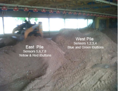
The farmer made a windrow approximately 3.70 m wide by 9.80 m long and 1.40 m high (about 25 m3). This consisted of approximately half the litter in the house (50 m x 10 m) and the crust had already been removed.
The litter was stacked longitudinally, though actually in more of a heap than a row down the whole length of the house, which created a higher pile. A large number of darkling beetles (Alphitobius diaperinus) were seen in the litter.
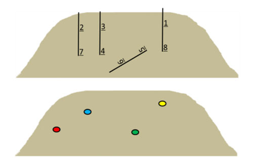
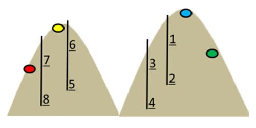
Equipment made by INTA was installed. This consisted of eight sensors, mounted on four wooden bars (two sensors per bar), on the south face of the pile, and four iButton data loggers on the north face.
Farm 1: results
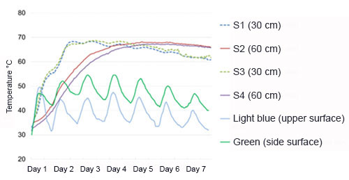
Figure 2 shows temperature changes during the windrow period. Sensors at similar depths can be seen to register similar temperatures.
For example, the sensors located closest to the surface, at a depth of 30 cm, detected the quickest temperature rise, peaking around day 2. In this group of sensors which registered the fastest increases, temperatures started to decrease slowly from the peak of about 70 °C.
It should be noted that the depth of the sensors changed from the moment that they were placed, due to compaction of the litter, which was very loose on windrowing and denser towards the end of the period. This caused variation in sensor depths throughout the process.
It should also be noted that the yellow sensor initially detected a rapid temperature rise which then decreased after day 2, as it had somehow been physically exposed, so measurements fluctuated in line with environmental temperature from day 3 onwards.
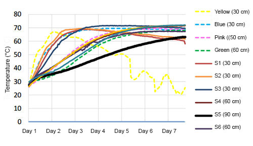
All the sensors at a depth of 60 cm behaved similarly, exceeding 60 °C from day 3 and increasing until near the end of the evaluation period. The 90 cm sensor, represented by the thicker black line on the graph, registered a much slower, gradual increase, possibly affected by proximity to the house floor.
Table 1 shows the physical, chemical and bacteriological characteristics of the poultry litter. The control sample was taken as the litter was windrowed, and the others when the sensors were removed.
Table 1. Results of physical, chemical and bacteriological analysis of the litter. Dry Matter (DM), pH, Electrical Conductivity (EC), Organic Carbon (C), Total Nitrogen (TN), Total Phosphorus (TP) and Carbon:Nitrogen Ratio (C:N). Measurement of Enterobacteria and sulphite-reducing anaerobes (CFU/g)* CFU/g = colony-forming units per gram.
|
Sample (sensor)
|
DM per cent
|
pH
|
EC (mS/cm)
|
C per cent
|
TN per cent
|
TP per cent
|
C:N
|
Entero bacteria CFU/g (*)
|
Sulphite-reducing anaerobes CFU/g
|
|---|---|---|---|---|---|---|---|---|---|
| Litter before windrowing |
70.40
|
8.4
|
12.37
|
47.0
|
2.67
|
0.63
|
17.60
|
2.7 x 10³
|
3.2 x 10²
|
| S1 (30 cm) |
76.54
|
8.2
|
14.40
|
47.7
|
2.75
|
0.72
|
17.35
|
10
|
-
|
| S2 (30 cm) |
75.87
|
8.1
|
15.34
|
46.6
|
4 x 10²
|
-
|
|||
| S3 (30 cm) |
74.08
|
8.1
|
14.58
|
48.1
|
-
|
-
|
|||
| S4 (60 cm) |
71.71
|
8.2
|
14.41
|
45.1
|
10
|
-
|
|||
| S5 (90 cm) |
74.98
|
8.5
|
13.77
|
47.9
|
-
|
1
|
|||
| S6 (60 cm) |
75.39
|
8.4
|
12.74
|
44.7
|
-
|
-
|
|||
| S7 (60 cm) |
74.13
|
7.6
|
14.84
|
46.2
|
-
|
-
|
|||
| S8 (60 cm) |
77.46
|
7.7
|
14.83
|
42.3
|
-
|
-
|
|||
| Pink (50 cm) |
70.48
|
7.5
|
14.70
|
47.4
|
-
|
-
|
|||
| Light blue (30 cm) |
68.24
|
8.4
|
15.11
|
45.7
|
2.96
|
0.69
|
15.78
|
-
|
-
|
| Yellow (30 cm) |
76.61
|
7.6
|
16.14
|
46.6
|
2.46
|
0.56
|
19.59
|
2.7 x 10²
|
-
|
| Green (50 cm) |
74.44
|
8.1
|
14.31
|
47.4
|
2.93
|
0.67
|
15.83
|
-
|
-
|
A significant reduction in the bacterial load was observed, as a result of the high temperatures generated inside the windrow, which indicates that the process was successful from a bird health perspective.
No clear trends were seen in relation to changes in pH, but an increase was detected in the EC, which was already higher than the levels indicated for the litter to be used as a fertiliser for intensive crops (Chilean legislation states that a good soil amendment should have values between 3 dS/m and 8 dS/m, whilst SENASA in Argentina establishes an EC value of less than 4 dS/m).
TP and TN were analysed to give an idea of the content of these elements, as poultry litter is mainly used for fertilising extensive crops, grazing and forage in the region. Firm conclusions can't be drawn from the limited data, but it seems that TP did not change, as was expected, but TN levels did.
TP values are low because the farmer removed the cake before stacking the litter, but TP levels in poultry litter are usually around 1.2-1.3 per cent.
Farm 1: conclusions
Windrowing reduced the bacterial load of poultry litter considerably under farm conditions.
Farm 2: details
The litter on this farm in the Department of Villaguay in Entre Rios was only used for one flock. Trial duration was seven days.
150 m x 12 m blackout house with side curtains, orientated east-west, wood shaving bedding, automatic feeders, nipple drinkers and tunnel ventilation (extractor fans).
The complete litter, as left at the end of the batch, was piled into a central windrow. No water was added by irrigation, and the cake (usually only a small amount) was also not tilled as the material was already loose enough.
Windrowing was carried out with a loader by the contractor who usually does this work on the farm. Broilers were being loaded in another part of the house as the windrowing was carried out.
On this occasion, unlike on Farm 1, the litter was piled in a windrow along the whole length of the house.
However, two piles of different sizes were made at one end of the house; one with a maximum height of 120 cm and the other adjoining pile, which continued the windrow to the end of the house, was a maximum of 90 cm high.
The data loggers were placed in the two piles, with the sensors attached to stakes at 30 cm and 60 cm depth, and the iButtons were placed 10 cm below the surface (Figure 3). The equipment was set to register the temperature every hour.
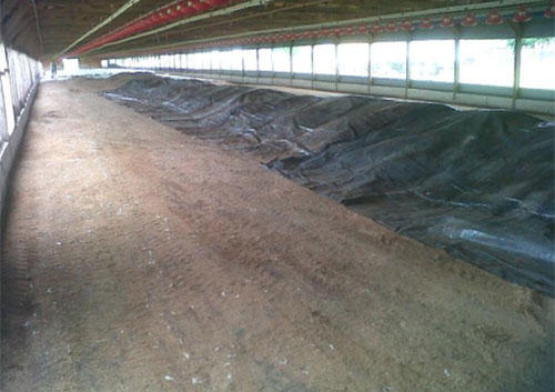
Another difference between this farm and Farm 1 was that the windrows were completely covered with low density black plastic once they were constructed and the sensors were placed.
Farm 2: results
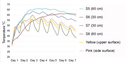
Figure 4 shows the temperatures detected by the sensors located in the taller row (120 cm). S1 and S3 (at a depth of 30 cm - dotted lines on the graph) registered faster temperature rises than S3 and S4 (60 cm deep). This was probably due to the effect of the temperature of the house floor on the deeper sensors.
The deepest points heated more slowly but tended to maintain temperature for longer, while those closest to the surface heated up sooner, but also started to cool quicker.
It was also noted that the deepest sensors did not register daily temperature fluctuations, while the sensors located at the surface of the pile, at a depth of 10 cm, did detect these changes.
In the case of the low pile (Figure 5), the temperatures registered by sensors S6 and S7 (30 cm deep) were quite different. This was because their depth was not maintained, so much so that S6 was almost at the surface of the pile when the equipment was removed.
The windrows shrunk noticeably during the process as the litter became compacted, so the original depth of the equipment was not maintained. S5 and S8 (60 cm deep) were also affected by this. S8 increased more gradually, slower even than the deep sensors in Figure 4, no doubt because of its proximity to the house floor, which slowed its warming. In contrast, S5 heated up faster and started to cool from day 4, like the 30 cm sensors, because it happened to be located on the bar where the windrow shrunk most (S5 was with S6, which was uncovered).
The shallower sensors (iButtons identified by yellow, light blue, pink and green colours) in both piles registered temperature fluctuations throughout the day, more exaggerated the closer the sensor was to the surface of the pile. In fact, the light blue iButton was discovered completely outside the tall pile, only covered by the plastic, when it was removed and it was this sensor that registered the lowest temperature.
As mentioned previously, S6 in the low pile had also come to the surface and it registered a similar pattern to the blue iButton. Although the temperature in the house was not recorded, its influence was obvious towards the edges of the windrow; the lowest temperatures occurred in the dawn hours and the highest in the afternoon.
It is important to note that the windrow surfaces were damp when the plastic was removed, as the temperature generated had evaporated the water from the interior which then condensed on the plastic. Covering with plastic also led to significant Alphitobius diaperinus beetle mortality.
Photo 4 shows an image taken with an infrared camera during the litter windrowing process, and the highest temperature point corresponds to the house floor where the litter had been spread until moments before, while the newly-formed windrow is colder, although the difference is only a few degrees centigrade.
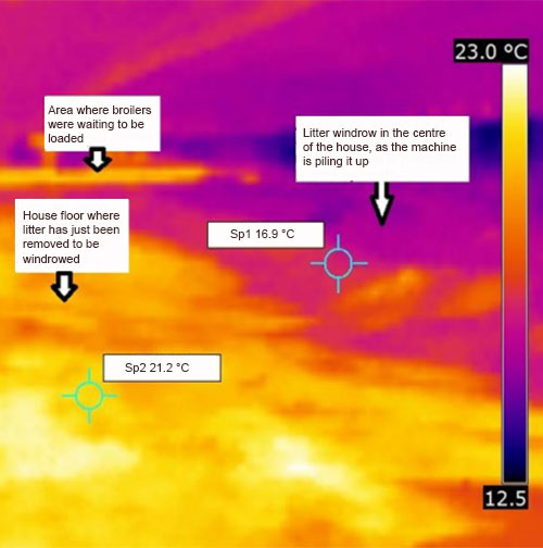
Photo 5 was taken as the pile was opened to remove the sensors, after 7 days of windrowing. One of the hottest points (53.5 °C) is highlighted and can be seen clearly. The other point highlighted shows the scoop used to extract samples. A blue tone (lower temperature) can be seen in the upper part of the image: this is the surface of the windrow.
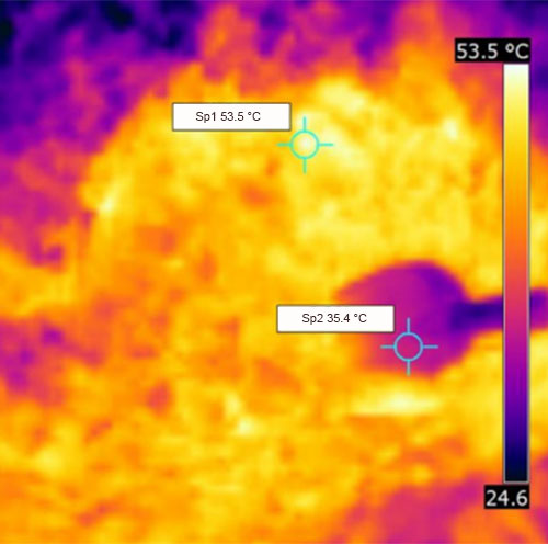
Table 2 shows the results of the physical, chemical and microbiological analysis of the litter. There was a noticeable reduction in enterobacteria and sulphite-reducing anaerobe counts from all locations in comparison with the control sample.
Table 2. Results of physical, chemical and bacteriological analysis of the litter. Dry Matter (DM), pH, Electrical Conductivity (EC), Organic Carbon (C), Total Nitrogen (TN), Total Phosphorus (TP) and Carbon:Nitrogen Ratio (C:N). Enterobacteria and sulphite-reducing anaerobes (CFU/g): (-) = level of bacteria too low to be detected by this technique. Control = sample taken before the windrowing process.
|
Sensor
| DM per cent | Moisture per cent | pH | EC | Entero bacteria CFU/g | Sulphite-reducing anaerobes CFU/g |
|---|---|---|---|---|---|---|
| Control |
72.6
|
27.4
|
8.22
|
8.050
|
6.4 x 10⁷
|
>300
|
| S1 |
75.8
|
24.2
|
8.35
|
7.650
|
-
|
-
|
| S2 |
69.5
|
30.5
|
7.89
|
12.075
|
-
|
-
|
| S3 |
71.8
|
28.2
|
8.00
|
9.765
|
-
|
-
|
| S4 |
56.1
|
43.9
|
8.02
|
19.025
|
-
|
-
|
| S5 |
87.3
|
12.7
|
8.38
|
7.985
|
-
|
-
|
| S6 |
78.4
|
21.6
|
8.09
|
10.985
|
-
|
-
|
| S7 |
75.6
|
24.4
|
8.29
|
6.735
|
-
|
-
|
| S8 |
69.7
|
30.3
|
7.54
|
11.825
|
-
|
-
|
| Yellow |
76.7
|
23.3
|
8.56
|
7.125
|
-
|
-
|
| Light blue |
67.5
|
32.5
|
7.91
|
14.905
|
25
|
-
|
| Pink |
65.9
|
34.1
|
8.29
|
12.635
|
-
|
40
|
| Green |
70.8
|
29.2
|
8.71
|
9.515
|
-
|
10
|
A significant variation in EC was observed (Coefficient of variation = 33 per cent), associated with the changes in moisture levels. EC values were higher than the control sample at some points and lower at others. In contrast to the windrow on Farm 1, moisture levels in this case were more variable, probably due to the effect of the plastic and the condensation it caused. There was no significant change in pH.
Outdoor windrow
Following on from previous experiments, and to fill some gaps in the information, samples were taken from the upper part (mostly cake) and lower part (the loose or tilled material beneath the cake) of the litter before windrowing to measure DM, TP, TN, pH and EC. Samples were composed of various 'nibbles' from different areas of the house.
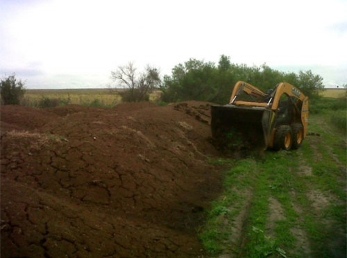
P y N levels are important from an agronomy perspective, as poultry litter is mainly used to fertilise extensive crops, grazing and forage in the area. This is why samples were taken from litter stacked outdoors on an arable plot near the farm. This pile had been used for about 6 flocks, was composed of wood shavings and had been stacked for at least two months (photo 6).
The upper surface was visibly wetter than the inside of the pile (photo 7). Samples were taken from both areas; the wetter surface and drier interior.
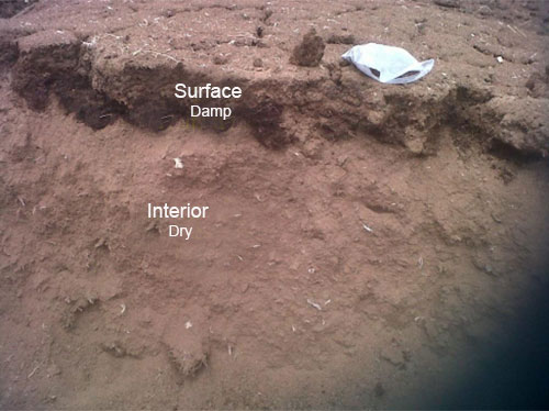
Table 3 shows the results of analysis of the litter in the various piles described above. Trends alone are observed, as the experiment was not replicated.
As predicted, both TN and TP levels were higher in the cake than the tilled poultry litter, while the sample from the pile after windrowing was a mixture of the two, and values were somewhere in between.
Comparison of the two samples from the outdoor pile shows that TN levels are similar, but P levels are higher in the wetter litter. pH and EC are also higher. Further investigation into this significant difference in TP is required.
Table 3. Results of physical and chemical analysis of the litter. Dry Matter (DM), pH, Electrical Conductivity (EC), Organic Carbon (C), Total Nitrogen (TN), Total Phosphorus (TP) and Carbon:Nitrogen Ratio (C:N). (*) DM, pH, EC and C analysed by the Agricultural Experimental Station at Concepción del Uruguay; TN and TP analysed by the Entre Ríos Cereals Arbitration Board.
|
Parameters (*)
|
DM per cent
|
pH
|
EC
|
C per cent
|
TN per cent
|
TP per cent
|
C:N
|
|---|---|---|---|---|---|---|---|
| Before treatment, Lower litter layer (loose) |
72.6
|
8.22
|
8.05
|
51.1
|
1.67
|
0.34
|
30.6
|
| Before treatment, Upper crust |
61.5
|
8.57
|
11.47
|
48.2
|
2.94
|
0.93
|
16.4
|
| After treatment, Sample from the pile |
56.6
|
8.715
|
10.15
|
43.73
|
2.08
|
0.38
|
21.02
|
| Stack on the arable plot, Lower layer, dry |
80.9
|
8.02
|
12.91
|
42
|
2.84
|
0.88
|
14.8
|
| Stack on the arable plot, Surface layer, damp |
41.5
|
8.72
|
>20
|
36.7
|
2.76
|
1.20
|
13.3
|
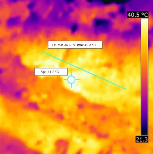
Photo 8 was taken with the infrared camera as the outdoor stack on the arable plot was opened. Although the pile had been stacked for 2 months, internal maximum values were still in excess of 40 °C.
Farm 2: conclusions
Windrowing under the conditions described reduced the bacterial load in poultry litter considerably. Levels of enterobacteria and sulphite-reducing anaerobes were reduced in the two piles (90 cm and 120 cm high respectively).
Different temperature patterns were recorded at different depths within the windrow. At the most superficial level (30 cm deep), increases were faster but lasted fewer days, while the temperature increased slower with more depth (60 cm) and was maintained until the end of the process.
The volume of the windrow decreased noticeably as the days passed, due to compaction. This was verified by the differences seen between the sensors theoretically located at the same depth.
Some results from the analysis of the different litter conditions (crust, tilled litter and stacked outdoors) call for more detailed study in order to start adapting farming methods.